How to Pull Data from Another Google Sheet: 6 Methods [2025]

Last Updated: December 23, 2025

‍

Getting data from one Google Sheet into another doesn't have to be complicated. Whether you're consolidating campaign reports from different clients or building a marketing dashboard that updates automatically, there's a method that fits your needs.

Quick answer: Use =Sheet1!A1 for pulling data within the same workbook, or =IMPORTRANGE("spreadsheet_url", "Sheet1!A1:D10") for external spreadsheets. For marketing data from platforms like Google Ads or Facebook, automation tools skip the formulas entirely.

This guide covers 6 methods from basic references to full automation—everything you need to stop manually copying data between sheets.

Quick Comparison

Method 1: Pull from Cells in the Same Sheet

The simplest method. Just reference the cell directly.

=B3

That's it. The value from B3 appears in your current cell and updates automatically when B3 changes.

When to use: Quick calculations, summary sections on the same tab.

To replicate down/across: Click the cell, grab the small blue square at the bottom-right corner, drag it in any direction. The formula adjusts automatically (B3 becomes B4, B5, etc.).

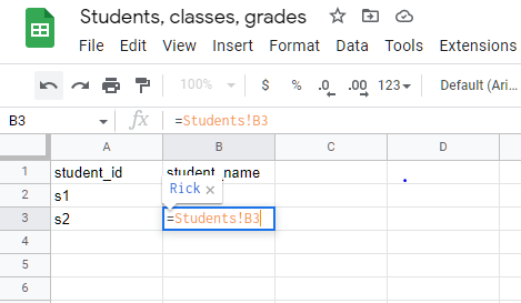
Method 2: Pull from Another Tab (Same Workbook)

When your data is on a different tab within the same Google Sheets file:

=Sheet1!A1

This pulls the value from cell A1 on "Sheet1."

If your sheet name has spaces or special characters, wrap it in single quotes:

='My Data Sheet'!A1
='Q4-2024'!A1

Real example: You have raw campaign data in a "Raw_Data" tab. Your dashboard pulls key metrics:

='Raw_Data'!B10

Common errors:

• #REF! = Sheet was renamed or deleted
• #NAME? = Forgot quotes around sheet name with spaces

Method 3: Pull Entire Ranges

Instead of writing 100 formulas for 100 rows, pull the entire range at once:

Specific range:

={A1:A100}

Entire column:

={A:A}

From another sheet:

={'Campaign Data'!A:E}

This is powerful for dashboards that need to stay in sync. When new campaigns get added to your source sheet, they automatically appear in your destination.

Performance tip: Entire column references (A:A) pull millions of potential rows. If you know your data ends at row 500, use A1:A500 instead.

Method 4: IMPORTRANGE for External Spreadsheets

When your source data is in a completely different Google Sheets file (different URL), use IMPORTRANGE.

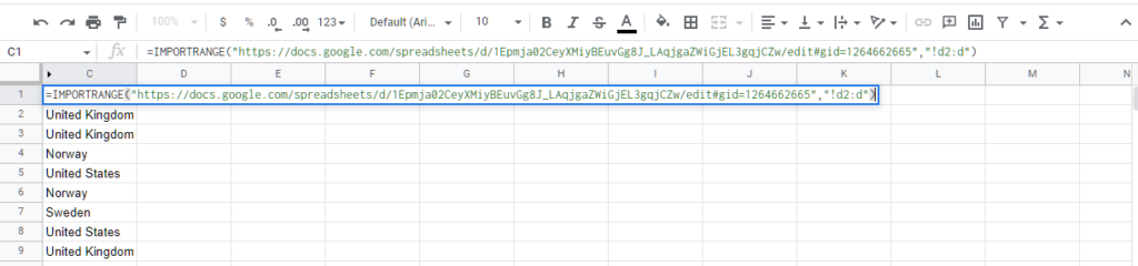
=IMPORTRANGE("https://docs.google.com/spreadsheets/d/1Abc...xyz", "Sheet1!A2:D100")

First-time setup:

1. Paste the formula
2. Click "Allow access" when prompted (one-time per source file)
3. Wait 30-60 seconds for initial load

Shorter syntax if pulling from first sheet:

=IMPORTRANGE("URL", "A2:D100")

Real Marketing Use Cases

Multi-client reporting:
Pull each client's data from their individual tracking sheets into your master report.

Regional consolidation:
Combine GA4 data from USA, UK, and EU properties into one analysis sheet.

Team collaboration:
Your team logs weekly progress in separate sheets. You IMPORTRANGE them all into a company overview.

IMPORTRANGE Limitations

Google has hard limits you should know about:

• Maximum 50 IMPORTRANGE functions per sheet (split across tabs if you need more)
• Slow with large datasets (1,000+ rows can take minutes)
• No guaranteed refresh timing (usually updates within 5-10 minutes)
• Requires permission for each new source file

Troubleshooting

"You need permission" → Click "Allow access" button

Loading forever → Reduce your range size. Try A1:Z100 instead of A:Z

#REF! error → Check that the URL and range are correct (copy URL from browser again)

Data not updating → IMPORTRANGE caches data. Edit the formula slightly (add a space), press Enter, then change it back to force refresh.

Google's official IMPORTRANGE documentation covers additional technical details and best practices.

Method 5: FILTER for Conditional Data

FILTER lets you pull only the rows that meet specific conditions. No more manually hiding rows or creating multiple sheets.

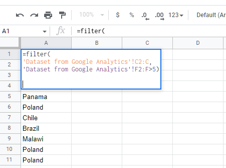
Basic syntax:

=FILTER(range, condition)

Example: Show only campaigns with more than 1,000 clicks:

=FILTER(A2:E100, C2:C100 > 1000)

This returns all rows where column C (clicks) is greater than 1,000.

Multiple Conditions

AND logic (both conditions must be true):

=FILTER(
 A2:E,
 (C2:C > 1000) * (D2:D = "Active")
)

The * means AND. This shows campaigns with >1,000 clicks AND "Active" status.

OR logic (either condition can be true):

=FILTER(
 A2:E,
 (D2:D = "Active") + (D2:D = "Testing")
)

The + means OR. Shows campaigns that are either Active OR Testing.

Combining FILTER with IMPORTRANGE

Pull filtered data from an external spreadsheet:

=FILTER(
 IMPORTRANGE("URL", "Data!A2:E"),
 IMPORTRANGE("URL", "Data!C2:C") > 100
)

Note: You must reference IMPORTRANGE twice—once for the data, once for the condition.

Error Handling

If no rows match your filter, you'll see "FILTER has no data to show." Add a fallback:

=IFERROR(
 FILTER(A2:E, C2:C > 100),
 "No campaigns meet criteria"
)

Learn more advanced filtering techniques in our complete FILTER function guide.

Method 6: QUERY for SQL-Like Operations

QUERY is the most powerful option. Think of it as SQL for Google Sheets.

Basic structure:

=QUERY(data, "query_string", headers)

Example: Pull specific columns where spend > $500:

=QUERY(
 Sheet1!A1:E100,
 "SELECT A, C, E WHERE D > 500 ORDER BY E DESC",
 1
)

This selects columns A, C, and E, filters where column D > 500, and sorts by column E descending.

Common QUERY Operations

Select specific columns:

=QUERY(A1:E, "SELECT A, C, E", 1)

Filter by text:

=QUERY(A1:E, "SELECT * WHERE B = 'Active'", 1)

Text values need single quotes.

Multiple conditions:

=QUERY(A1:E, "SELECT * WHERE C > 1000 AND D = 'Active'", 1)

Sort results:

=QUERY(A1:E, "SELECT * ORDER BY E DESC LIMIT 10", 1)

Group and aggregate:

=QUERY(A1:D, "SELECT A, SUM(D) GROUP BY A", 1)

QUERY with IMPORTRANGE

Pull and transform data from external sheets:

=QUERY(
 IMPORTRANGE("URL", "Campaigns!A1:E"),
 "SELECT Col1, Col3, Col5 WHERE Col4 > 500",
 1
)

When using IMPORTRANGE inside QUERY, use Col1, Col2, etc. instead of A, B, C.

Real Scenario: Consolidate Multiple Sources

You have 3 regional sheets with campaign data. Pull everything with spend >$500:

=QUERY(
 {
   IMPORTRANGE("URL1", "Sheet1!A2:E");
   IMPORTRANGE("URL2", "Sheet1!A2:E");
   IMPORTRANGE("URL3", "Sheet1!A2:E")
 },
 "SELECT * WHERE Col4 > 500 ORDER BY Col5 DESC",
 0
)

Use 0 for headers when combining multiple sources (prevents duplicate headers).

When to use QUERY:

• Complex filtering (multiple AND/OR conditions)
• Data aggregation (SUM, AVG, COUNT)
• SQL-like operations
• Combining multiple sources

When to use FILTER instead:

• Simple conditions
• Want entire row result
• Prefer simpler syntax

For more QUERY examples specific to marketing data, check out our Google Sheets QUERY function guide.

Method 7: Automate Marketing Data with Dataslayer

All the methods above work for pulling data between Google Sheets. But what about pulling data from advertising platforms like Google Ads, Facebook, or LinkedIn into Sheets?

That's where manual exports become a bottleneck—and where automation saves hours.

The Manual Problem

Typical weekly workflow without automation:

1. Open Google Ads → Export to CSV
2. Upload to Google Sheets
3. Open Facebook Ads → Export to CSV
4. Upload to Google Sheets
5. Open LinkedIn Ads → Export to CSV
6. Upload to Google Sheets
7. Use IMPORTRANGE to consolidate
8. Fix broken formulas from format changes
9. Repeat next week

Time cost: 45-90 minutes per week
Error rate: High (manual copy-paste mistakes)

The Automated Approach

With Dataslayer:

1. Install add-on (one time)
2. Select data source (Google Ads, Facebook, etc.)
3. Choose metrics and date range
4. Click "Get Data"
5. Schedule daily/weekly refresh
6. Done forever

Time cost: 10 minutes setup, then automatic
Error rate: Zero (direct API connection)

Setup in 5 Steps

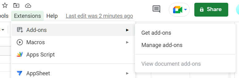
Step 1: Install from Google Workspace Marketplace

In Google Sheets:

• Extensions → Add-ons → Get add-ons
• Search "Dataslayer"
• Install

Step 2: Launch sidebar

Extensions → Dataslayer → Launch sidebar

Step 3: Connect your platform

• Select data source (e.g., "Google Ads")
• Authenticate with your account
• Select which account if you have multiple

Step 4: Configure your data

Pick metrics: Clicks, Impressions, Cost, Conversions, etc.
Pick dimensions: Campaign, Date, Device, etc.
Set date range: Last 7 days, Last 30 days, Custom, etc.

Step 5: Get data & schedule

• Click "Get Data to Table"
• Data appears instantly
• Click "Schedule Refresh" → Choose frequency
• Set it to daily at 8 AM and forget about it

Real Use Case Examples

Agency with 10 Google Ads clients:

Manual method: 60+ minutes daily (10 logins, 10 exports, 10 uploads)
Dataslayer: 50 minutes setup (one time), then 0 minutes daily
Time saved: 20+ hours per month

Cross-platform dashboard:

Need: Google Ads + Facebook Ads + LinkedIn Ads in one view
Manual: 3 separate exports, format reconciliation, broken formulas
Dataslayer: One query per platform, standardized data, automatic updates
Benefit: Direct platform comparison without format headaches

Client reporting:

15 clients need weekly reports
Manual: 3+ hours every Monday pulling fresh data
Dataslayer: Schedule refresh Monday 7 AM, reports ready before work starts
Time saved: 12+ hours per month

Dataslayer vs Manual Methods

When to Use Dataslayer

✓ You regularly pull data from ad platforms
✓ You manage multiple client accounts
✓ You need cross-platform reporting
✓ You value time over manual work
✓ You want zero-maintenance automation

Pricing Consideration

If you spend 1 hour daily on manual data pulls, that's ~20 hours monthly. At any professional rate, automation pays for itself immediately.

Try Dataslayer free for 15 days →

Dataslayer also works with Looker Studio, BigQuery, Power BI, and more. Same easy setup, different destinations. Learn more about automating Google Sheets data workflows.

Common Errors and Quick Fixes

#REF! Error

Cause: Reference is broken
Fix: Check that sheet name is spelled correctly. Use quotes for names with spaces: ='My Sheet'!A1

#NAME? Error

Cause: Google Sheets doesn't recognize something
Fix: Check function spelling. Add quotes around sheet names with special characters.

"You need permission to access"

Cause: IMPORTRANGE needs authorization
Fix: Click the blue "Allow access" button. You need at least View access to the source sheet.

"Loading..." Forever

Cause: Dataset too large or connection slow
Fix: Reduce range size. Change A:Z to A1:Z1000. Test with smaller range first.

IMPORTRANGE Returns Blank

Cause: Range is empty or incorrect
Fix: Open source sheet and verify data exists. Try a simple test range like A1:B5 first.

FILTER Has No Data

Cause: No rows meet your conditions
Fix: This isn't always an error. Add fallback: =IFERROR(FILTER(...), "No results")

Data Not Updating

Cause: IMPORTRANGE caches data (5-10 minute refresh)
Fix: Force refresh by editing formula slightly, press Enter, then change it back. Or check: File → Settings → Calculation → "On change and every minute"

For more troubleshooting, see Google's official help docs.

Best Practices

1. Use Named Ranges

Instead of =Sheet1!A1:A100, name the range "CampaignNames" and use =Sheet1!CampaignNames.

Benefits: Easier to read, update once to change everywhere, less prone to errors.

2. Limit IMPORTRANGE Usage

Google's limit: 50 per sheet. Each one adds load time.

Better: Pull all needed data in one IMPORTRANGE, then reference columns from that import.

3. Specify Exact Ranges

=IMPORTRANGE("URL", "A:Z") pulls potentially millions of rows.
=IMPORTRANGE("URL", "A1:Z500") is much faster.

4. Test Small First

Before pulling 10,000 rows, test with 10:
=IMPORTRANGE("URL", "A1:E10")

Verify it works, then expand the range.

5. Add Error Handling

Wrap important formulas:

=IFERROR(
 IMPORTRANGE("URL", "Data!A1:D100"),
 "Unable to load data"
)

6. Document Your Data Flow

Create a "Documentation" sheet explaining:

• Where data comes from
• Who maintains each connection
• Update frequency
• Contact for questions

This saves hours when someone leaves or formulas break.

Choosing the Right Method

Same sheet, single cells → Use =A1

Same workbook, different tabs → Use =Sheet1!A1

External spreadsheets → Use IMPORTRANGE

Need filtering → Use FILTER for simple conditions, QUERY for complex

Marketing platform data → Use automation tools like Dataslayer

The simplest method that solves your problem is the right method.

Next Steps

Continue learning:

• Connect Google Ads to Google Sheets - Automate Google Ads reporting
• Google Sheets QUERY Function: 15 Formulas - Master advanced queries
• FILTER Function Complete Guide - Deep dive into filtering
• Google Sheets Automation Guide - Automate everything
• Google Sheets Templates - Ready-to-use templates

Frequently Asked Questions

How do I pull data from another Google Sheet automatically?
Use =IMPORTRANGE("spreadsheet_url", "Sheet1!A1:D10") for external sheets. It updates automatically when source data changes, though refresh can take 5-10 minutes.

What's the difference between FILTER and QUERY?
FILTER is simpler and returns full rows based on conditions. QUERY is more powerful, letting you select specific columns, aggregate data, and use SQL-like syntax. See detailed comparison here.

Can I pull data from Google Ads into Google Sheets?
Yes, either using Google's official add-on or automation tools like Dataslayer. See complete setup guide.

How many IMPORTRANGE functions can I use?
Google limits you to 50 IMPORTRANGE functions per sheet. If you need more, split across multiple tabs or consolidate your imports.

Why is my IMPORTRANGE loading forever?
Large datasets (1,000+ rows) can timeout. Reduce your range size from A:Z to something specific like A1:Z500. Also check that the source sheet doesn't have calculation errors.

Questions about pulling data in Google Sheets? Contact our support team or check our Knowledge Base for more tutorials.